Random Points in a Circle

Here’s a problem: How do you get a uniform distribution of points in a circle? The solution for a square is pretty simple: you take a random $x$ and a random $y$ and you get a point $(x, y)$!

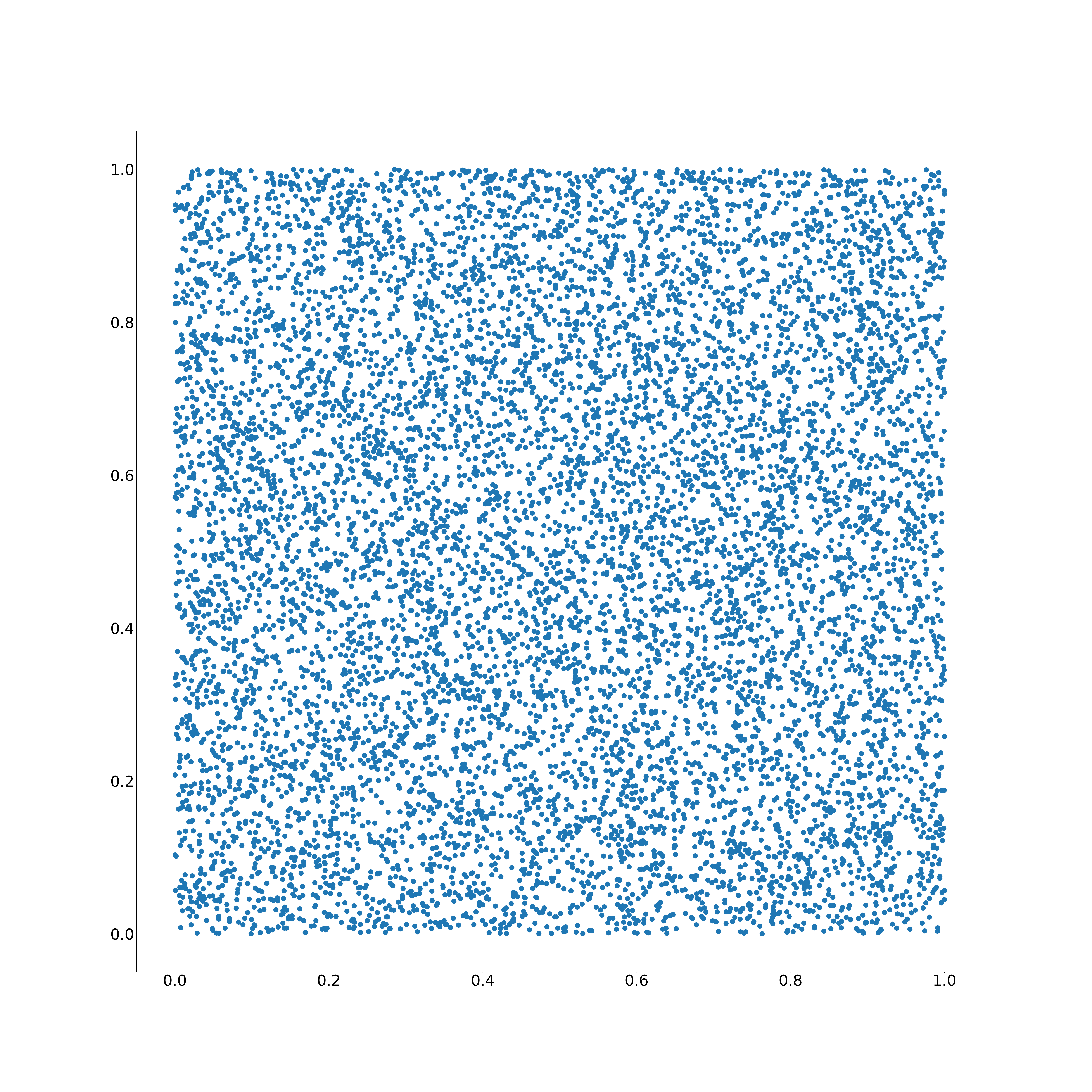
$(x, y)$ = (random(), random())

A naive idea for a circle might be to use this approach, but ignore everything not in it (e.g. ignore every point where $ 1 \lt \sqrt{x^2 + y^2}$).

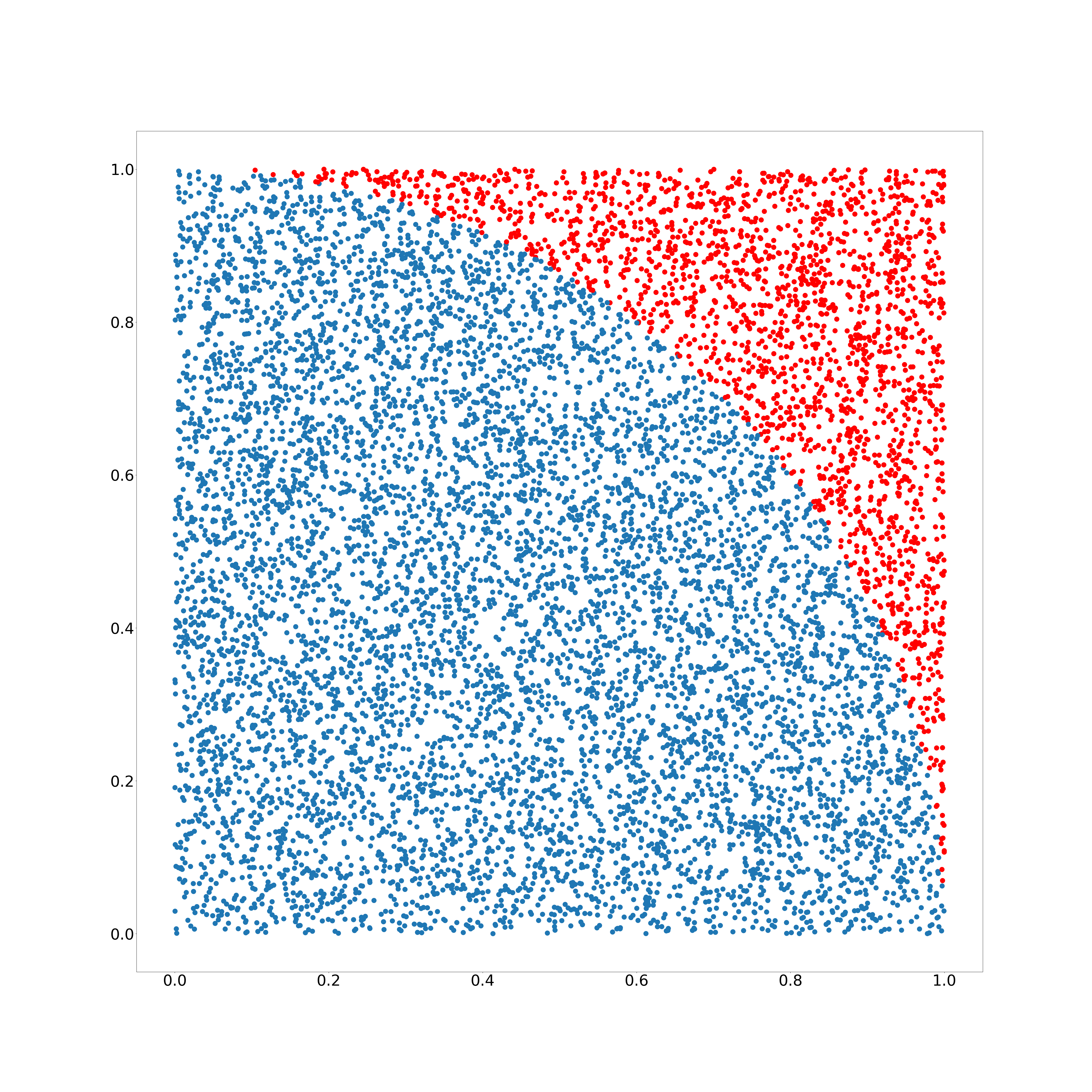
$(x, y)$ = (random(), random()), circle coloured

However, this isn’t very efficient: You loose more than 20% of your points! ^[1]

Maybe another coordinate system helps: polar coordinates use a radius and an angle, $(r, \varphi)$.

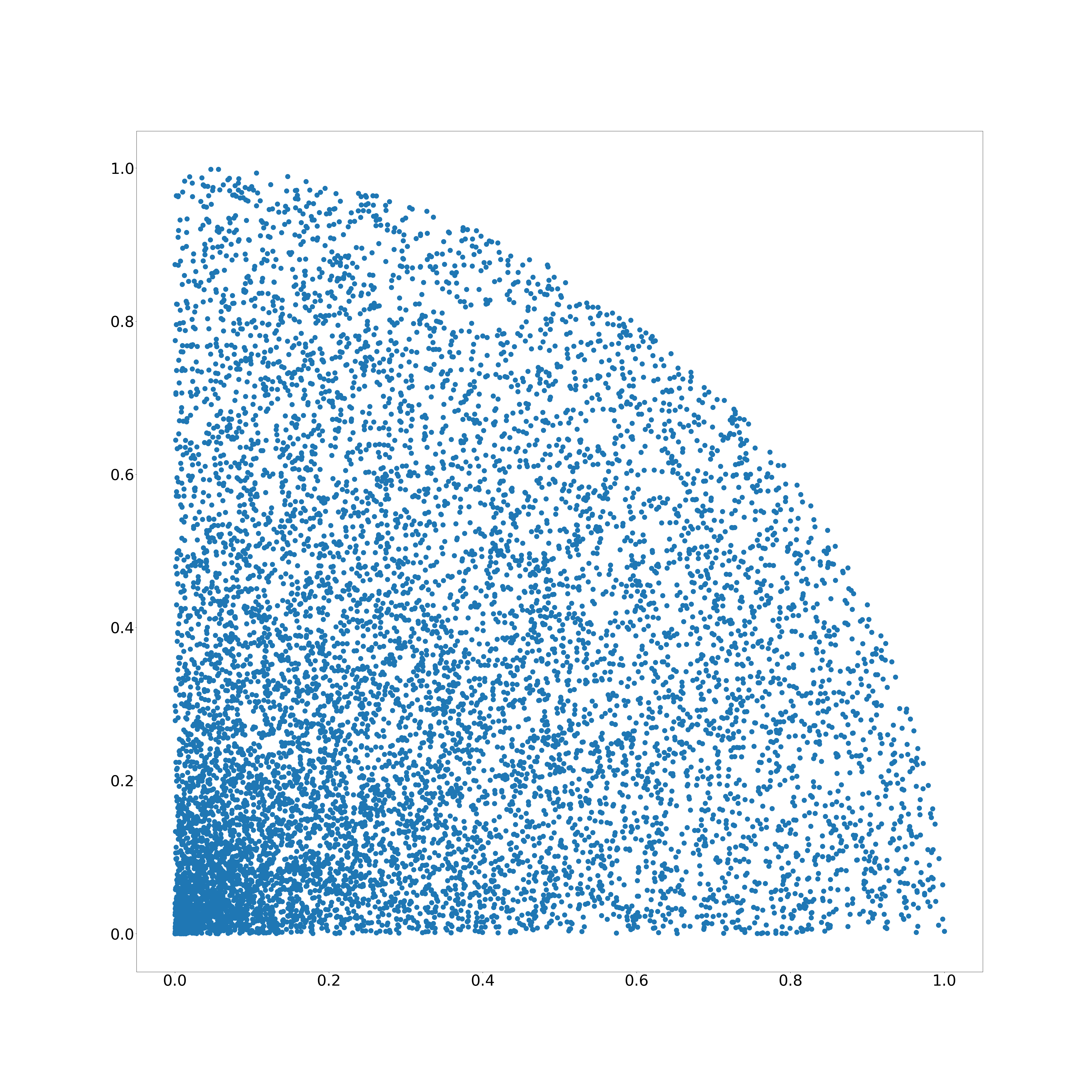
$(r, \varphi)$ = (random(), random() * $0.5  \pi$)

This doesn’t work: a random radius and a random angle don’t create a uniform distribution. Why is that?

On every line between the centre and the edge of the circle are approximately equal points, since a point’s angle is randomly chosen. The same is true for every circle perimeter, since the radius is random as well.

Here is the problem: when the radius becomes larger, the perimeter becomes larger as well, but maintains the number of points. This leads to a decrease in point density, since the distance between those points increases. ^[2]

The solution is to take the square root of the radius.

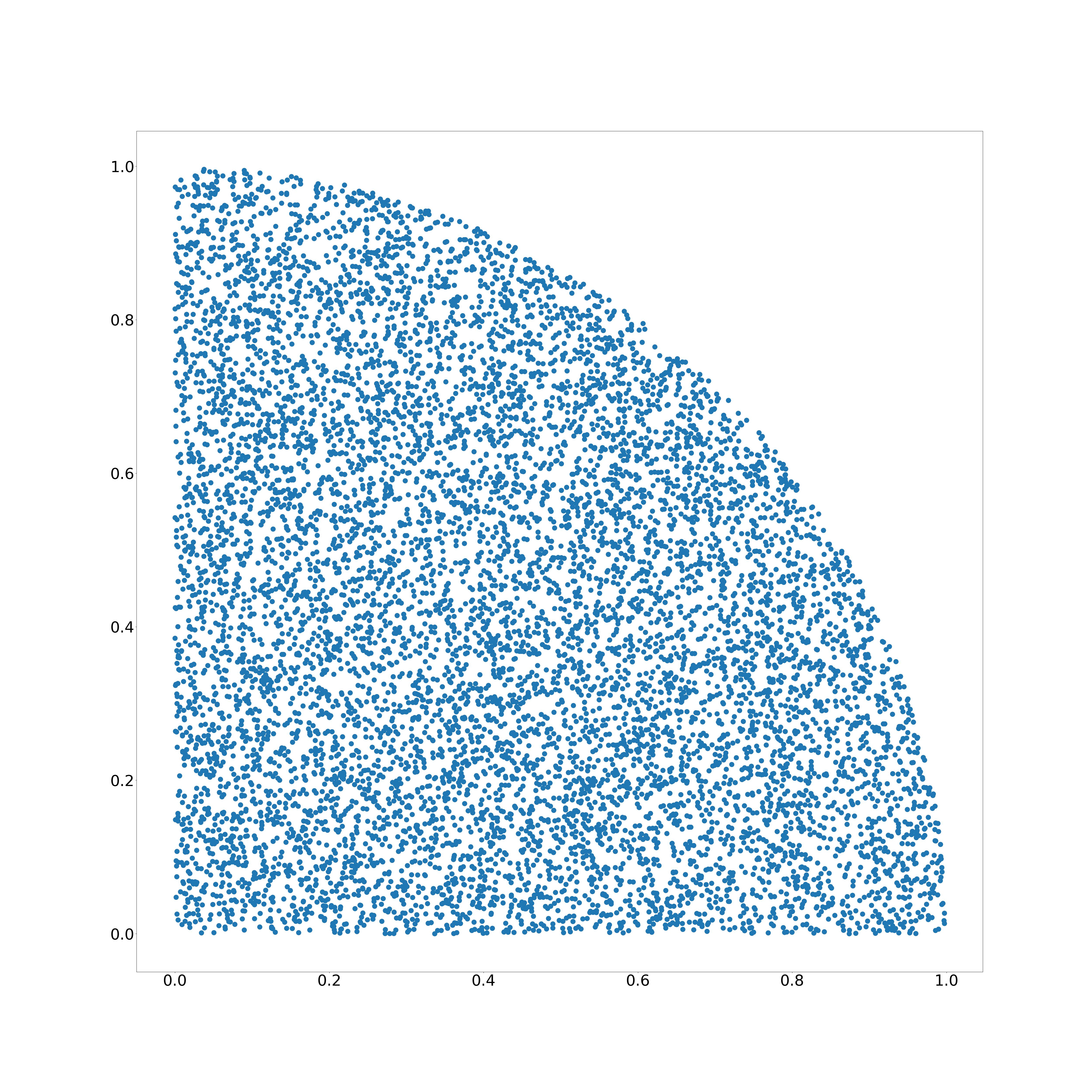
$(r, \varphi)$ = (sqrt(random()), random() * $0.5 \pi$)

Why does that work? A probability density function (PDF) provides the probability of a random value being in a chosen interval. Until now, our PDF was constant ($f(r) = a$), since every radius $r$ had an equal probability of occuring. The number of points in each radius interval was therefore constant as well.

However, since the perimeter of a circle grows linearly ($2r\pi$), our PDF has to grow linearly as well to keep the density of points (instead of the number of points) constant. The most important characteristics of a PDF are that it is non-negative and that the integral of the function from $-\infty$ to $+\infty$ is 1.

We therefore need a function with an integral that is 1 between 0 and the radius $R$ of the circle. $f(r) = r$ doesn’t work: $ \int_0^R f(r) dr = R^2 / 2 = 0.5$ (with $R = 1$), but the solution is simple: $f(r) = 2r/R^2$ and therefore $F(x) = \int_0^x f(r) dr = x^2 / R^2$ as our distribution function.

While a probability density function provides the probability of a random value being in a chosen interval, a distribution function calculates the probability of a value being less or equal than a given $x$.

If we invert the distribution function, it doesn’t calculate the probability of a value being less or equal to $x$, but gives the largest possible $x$ for a given probability.

$$ F^{-1}(x): x = \frac{y^2}{R^2} $$ $$ y^2 = R^2 * x $$ $$ y = \sqrt{R^2 * x} $$ $$ F^{-1}(x) = R * \sqrt{x} $$

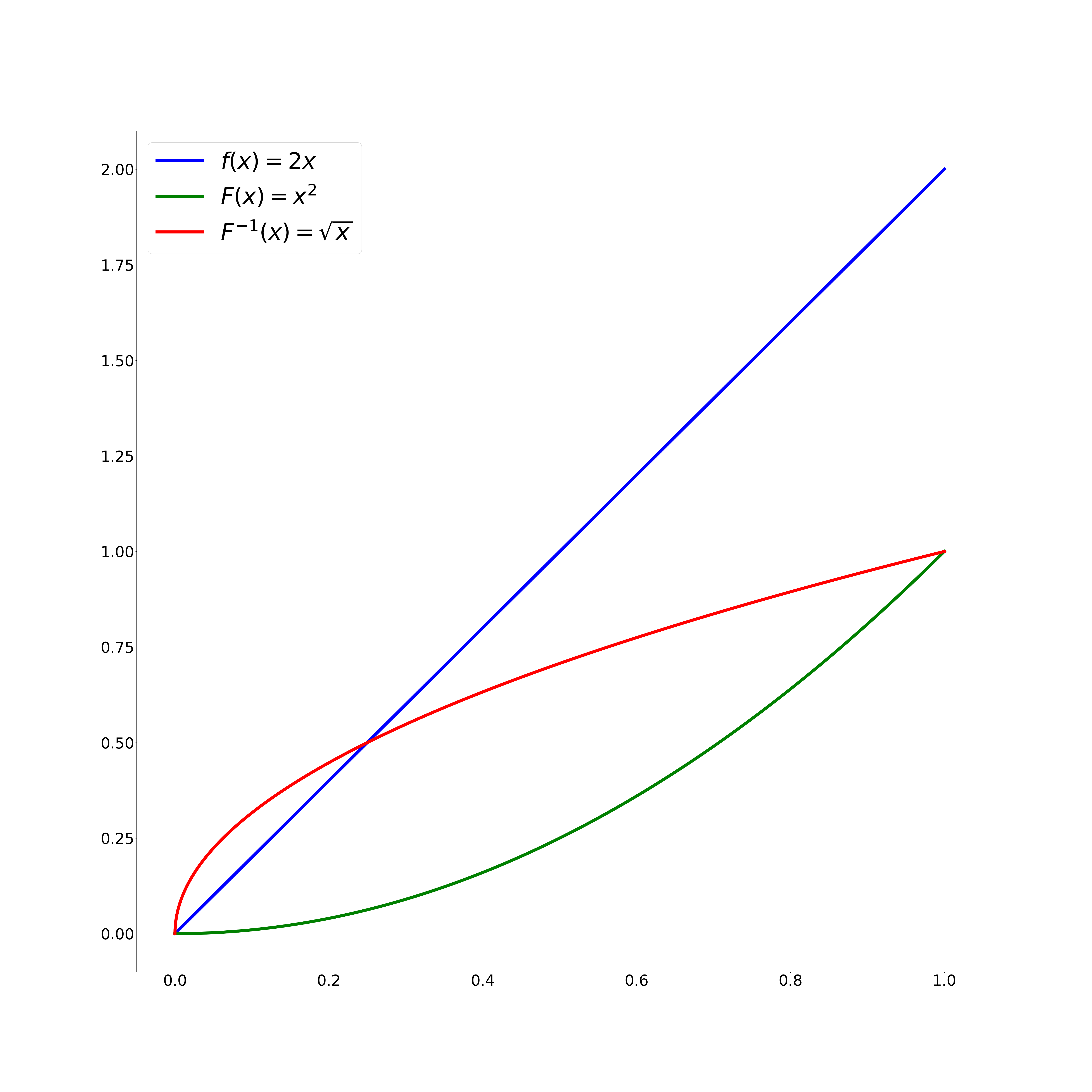
The graphs of the used functions

If we take this biggest possible value as the actual value of the coordinate radius, we get a uniform distribution of points in a circle.

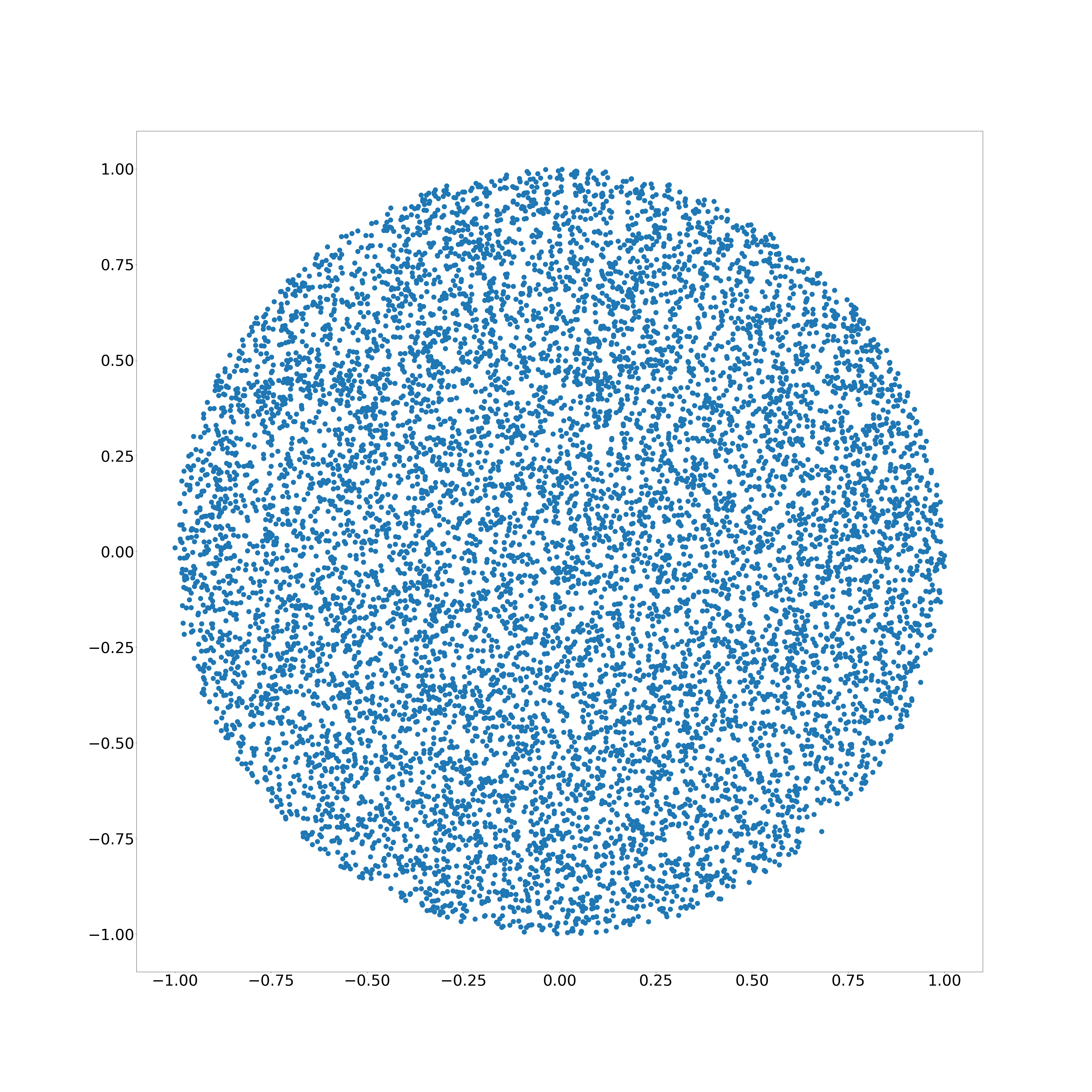
$(r, \varphi)$ = (sqrt(random()), random() * $2 \pi$)